Itō's lemma

In mathematics, Itō's lemma is used in Itō stochastic calculus to find the differential of a function of a particular type of stochastic process. It is named after its discoverer, Kiyoshi Itō. It is the stochastic calculus counterpart of the chain rule in ordinary calculus and is best memorized using the Taylor series expansion and retaining the second order term related to the stochastic component change. The lemma is widely employed in mathematical finance and its best known application is in the derivation of the Black–Scholes equation used to value options. Ito's Lemma is also referred to currently as the Itō–Doeblin Theorem in recognition of the recently discovered work of Wolfgang Doeblin.^[1]

1 Mathematical formulation of Itō's lemma
2 Informal derivation
3 Examples
4 See also
5 Notes
6 References
7 External links

Mathematical formulation of Itō's lemma

In the following subsections we discuss versions of Itō's lemma for different types of stochastic processes.

Itō drift-diffusion processes

In its simplest form, Itō's lemma states the following: for an Itō drift-diffusion process

$dX_t= \mu_t\,dt %2B \sigma_t\,dB_t$

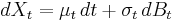
and any twice differentiable function ƒ(t, x) of two real variables t and x, one has

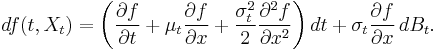
$\begin{align} df(t,X_t) =\left(\frac{\partial f}{\partial t} %2B \mu_t \frac{\partial f}{\partial x} %2B \frac{\sigma_t^2}{2}\frac{\partial^2f}{\partial x^2}\right)dt%2B \sigma_t \frac{\partial f}{\partial x}\,dB_t. \end{align}$

This immediately implies that ƒ(t, X) is itself an Itō drift-diffusion process.

In higher dimensions, Ito's lemma states

$df\left( t,X_t \right)=\dot{f}_t \left(t,X_t \right)\,dt %2B \nabla_{X_t}^T f\cdot dX_t %2B \frac{1}{2} \, dX^T_t \cdot\nabla_{X_t}^2 f\cdot dX_t$

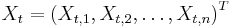where $X_t =\left( X_{t,1}, X_{t,2}, \ldots, X_{t,n} \right)^T$ is a vector of Itō processes, $\dot{f}_t \left(t,X\right)$ is the partial differential w.r.t. t, $\nabla_{X}^T f$ is the gradient of ƒ w.r.t. X, and $\nabla_{X}^2 f$ is the Hessian matrix of ƒ w.r.t. X.

Continuous semimartingales

More generally, the above formula also holds for any continuous d-dimensional semimartingale X = (X¹,X²,…,X^d), and twice continuously differentiable and real valued function f on R^d. Some people prefer to present the formula in another form with cross variation shown explicitly as follows, f(X) is a semimartingale satisfying

$df(X_t) = \sum_{i=1}^d f_{i}(X_t)\,dX^i_t %2B \frac{1}{2}\sum_{i,j=1}^df_{i,j}(X_t)\,d[X^i,X^j]_t.$

In this expression, the term f_i represents the partial derivative of f(x) with respect to xⁱ, and [Xⁱ,X^j ] is the quadratic covariation process of Xⁱ and X^j.

Poisson jump processes

We may also define functions on discontinuous stochastic processes.

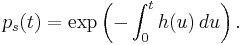
Let h be the jump intensity. The Poisson process model for jumps is that the probability of one jump in the interval $[t, t %2B \Delta t]$ is $h \Delta t$ plus higher order terms. h could be a constant, a deterministic function of time, or a stochastic process. The survival probability $p_s(t)$ is the probability that no jump has occurred in the interval $[0,t]$ . The change in the survival probability is

$d p_s(t) = -p_s(t) h(t) \, dt.$

$p_s(t) = \exp \left(-\int_0^t h(u) \, du \right).$

Let $S(t)$ be a discontinuous stochastic process. Write $S(t^-)$ for the value of S as we approach t from the left. Write $d_j S(t)$ for the non-infinitesimal change in $S(t)$ as a result of a jump. Then

$d_j S(t)=\lim_{\Delta t \to 0}(S(t%2B\Delta t)-S(t^-))$

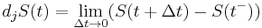
Let z be the magnitude of the jump and let $\eta(S(t^-),z)$ be the distribution of z. The expected magnitude of the jump is

$E[d_j S(t)]=h(S(t^-)) \, dt \int_z z \eta(S(t^-),z) \, dz.$

Define $d J_S(t)$ , a compensated process and martingale, as

$d J_S(t)=d_j S(t)-E[d_j S(t)]=S(t)-S(t^-)-(h(S(t^-)) \int_z z \eta(S(t^-),z) \, dz) \, dt.$

Then

$d_j S(t) = E[d_j S(t)] %2B d J_S(t) = h(S(t^-)) (\int_z z \eta(S(t^-),z) \, dz) dt %2B d J_S(t).$

Consider a function $g(S(t),t)$ of jump process $d S(t)$ . If $S(t)$ jumps by $\Delta s$ then $g(t)$ jumps by $\Delta g$ . $\Delta g$ is drawn from distribution $\eta_g()$ which may depend on $g(t^-)$ , dg and $S(t^-)$ . The jump part of $g$ is

$\begin{align} g(t)-g(t^-) & =h(t) \, dt \int_{\Delta g} \, \Delta g \eta_g(\cdot) \, d\Delta g %2B d J_g(t). \end{align}$

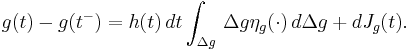
If $S$ contains drift, diffusion and jump parts, then Itō's Lemma for $g(S(t),t)$ is

$\begin{align} d g(t) & = \left( \frac{\partial g}{\partial t}%2B\mu \frac{\partial g}{\partial S}%2B\frac{1}{2} \sigma^2 \frac{\partial^2 g}{\partial S^2}%2Bh(t)\int_{\Delta g} (\Delta g \eta_g(\cdot) \, d{\Delta}g) \, \right) dt %2B \frac{\partial g}{\partial S} \sigma \, d W(t) %2B d J_g(t). \end{align}$

Itō's lemma for a process which is the sum of a drift-diffusion process and a jump process is just the sum of the Itō's lemma for the individual parts.

Non-continuous semimartingales

Itō's lemma can also be applied to general d-dimensional semimartingales, which need not be continuous. In general, a semimartingale is a càdlàg process, and an additional term needs to be added to the formula to ensure that the jumps of the process are correctly given by Itō's lemma. For any cadlag process Y_t, the left limit in t is denoted by Y_t-, which is a left-continuous process. The jumps are written as ΔY_t = Y_t - Y_t-. Then, Itō's lemma states that if X = (X¹,X²,…,X^d) is a d-dimensional semimartingale and f is a twice continuously differentiable real valued function on R^d then f(X) is a semimartingale, and

$\begin{align} f(X_t)= & f(X_0)%2B\sum_{i=1}^d\int_0^t f_{i}(X_{s-})\,dX^i_s %2B \frac{1}{2}\sum_{i,j=1}^d \int_0^t f_{i,j}(X_{s-})\,d[X^i,X^j]_s\\ &{} %2B \sum_{s\le t}\left(\Delta f(X_s)-\sum_{i=1}^df_{i}(X_{s-})\,\Delta X^i_s-\frac{1}{2}\sum_{i,j=1}^d f_{i,j}(X_{s-})\,\Delta X^i_s \, \Delta X^j_s\right). \end{align}$

This differs from the formula for continuous semimartingales by the additional term summing over the jumps of X, which ensures that the jump of the right hand side at time t is Δf(X_t).

Informal derivation

A formal proof of the lemma requires us to take the limit of a sequence of random variables, which is not done here. Instead, we give a sketch of how one can derive Itō's lemma by expanding a Taylor series and applying the rules of stochastic calculus.

Assume the Itō process is in the form of

$dx= a\,dt %2B b\,dB.\!$

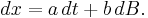
Expanding f(x, t) in a Taylor series in x and t we have

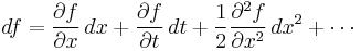
$df = \frac{\partial f}{\partial x}\,dx %2B \frac{\partial f}{\partial t}\,dt %2B \frac{1}{2}\frac{\partial^2 f}{\partial x^2}\,dx^2 %2B \cdots$

and substituting a dt + b dB for dx gives

$df = \frac{\partial f}{\partial x}(a\,dt %2B b\,dB) %2B \frac{\partial f}{\partial t}\,dt %2B \frac{1}{2}\frac{\partial^2 f}{\partial x^2}(a^2\,dt^2 %2B 2ab\,dt\,dB %2B b^2\,dB^2) %2B \cdots.$

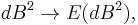
In the limit as dt tends to 0, the dt² and dt dB terms disappear but the dB² term tends to dt. The latter can be shown if we prove that

$dB^2 \rightarrow E(dB^2),$ since $E(dB^2) = dt. \,$

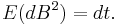
Deleting the dt² and dt dB terms, substituting dt for dB², and collecting the dt and dB terms, we obtain

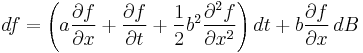
$df = \left(a\frac{\partial f}{\partial x} %2B \frac{\partial f}{\partial t} %2B \frac{1}{2}b^2\frac{\partial^2 f}{\partial x^2}\right)dt %2B b\frac{\partial f}{\partial x}\,dB$

as required.

The formal proof is somewhat technical and is beyond the current state of this article.

Examples

Geometric Brownian motion

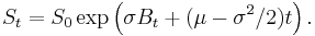
A process S is said to follow a geometric Brownian motion with volatility σ and drift μ if it satisfies the stochastic differential equation dS = S(σdB + μdt), for a Brownian motion B. Applying Itō's lemma with f(S) = log(S) gives

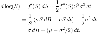
$\begin{align} d\log(S) & = f^\prime(S)\,dS %2B \frac{1}{2}f^{\prime\prime} (S)S^2\sigma^2 \,dt \\ & = \frac{1}{S} \left( \sigma S\,dB %2B \mu S\,dt\right) - \frac{1}{2}\sigma^2\,dt \\ &= \sigma\,dB %2B(\mu-\sigma^2/2)\,dt. \end{align}$

It follows that log(S_t) = log(S₀) + σB_t + (μ − σ²/2)t, and exponentiating gives the expression for S,

$S_t=S_0\exp\left(\sigma B_t%2B(\mu-\sigma^2/2)t\right).$

The Doléans exponential

The Doléans exponential (or stochastic exponential) of a continuous semimartingale X can be defined as the solution to the SDE dY = Y dX with initial condition Y₀ = 1. It is sometimes denoted by Ɛ(X). Applying Itō's lemma with f(Y) = log(Y) gives

$\begin{align} d\log(Y) &= \frac{1}{Y}\,dY -\frac{1}{2Y^2}\,d[Y] \\ &= dX - \frac{1}{2}\,d[X]. \end{align}$

Exponentiating gives the solution

$Y_t = \exp\left(X_t-X_0-[X]_t/2\right).$

Black–Scholes formula

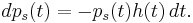
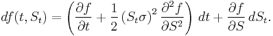
Itō's lemma can be used to derive the Black–Scholes formula for an option. Suppose a stock price follows a Geometric Brownian motion given by the stochastic differential equation dS = S(σdB + μ dt). Then, if the value of an option at time t is f(t,S_t), Itō's lemma gives

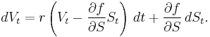
$df(t,S_t) = \left(\frac{\partial f}{\partial t} %2B \frac{1}{2}\left(S_t\sigma\right)^2\frac{\partial^2 f}{\partial S^2}\right)\,dt %2B\frac{\partial f}{\partial S}\,dS_t.$

The term (∂f/∂S) dS represents the change in value in time dt of the trading strategy consisting of holding an amount ∂f/∂S of the stock. If this trading strategy is followed, and any cash held is assumed to grow at the risk free rate r, then the total value V of this portfolio satisfies the SDE

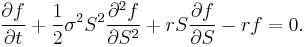
$dV_t = r\left(V_t-\frac{\partial f}{\partial S}S_t\right)\,dt %2B \frac{\partial f}{\partial S}\,dS_t.$

This strategy replicates the option if V = f(t,S). Combining these equations gives the celebrated Black-Scholes equation

$\frac{\partial f}{\partial t} %2B \frac{1}{2}\sigma^2S^2\frac{\partial^2 f}{\partial S^2} %2B rS\frac{\partial f}{\partial S}-rf = 0.$

Notes

^ "Stochastic Calculus :: Itô–Döblin formula", Michael Stastny

References

Kiyoshi Itō (1951). On stochastic differential equations. Memoirs, American Mathematical Society 4, 1–51.
Hagen Kleinert (2004). Path Integrals in Quantum Mechanics, Statistics, Polymer Physics, and Financial Markets, 4th edition, World Scientific (Singapore); Paperback ISBN 981-238-107-4. Also available online: PDF-files. This textbook also derives generalizations of Itō's lemma for non-Wiener (non-Gaussian) processes.
Bernt Øksendal (2000). Stochastic Differential Equations. An Introduction with Applications, 5th edition, corrected 2nd printing. Springer. ISBN 3-540-63720-6. Sections 4.1 and 4.2.
Domingo Tavella (2002). Quantitative Methods in Derivatives Pricing: An Introduction to Computational Finance, John Wiley and Sons. ISBN 9780471274797. Pages 36–39.

External links

Derivation, Prof. Thayer Watkins
Informal proof, optiontutor